Omicron Research Institute
QuanTek Econometric & Technical Analysis Software
QuanTek Price Projection
Normal types of technical indicators, such as for example moving averages, are functions of past prices or returns that are supposed to have predictive power for the future price action. For example, an exponentially weighted moving average (EWMA) of returns can be used as a predictor of future returns, which assumes a certain (stationary) correlation between past and future returns. According to Harvey, the EWMA is the optimal Linear Prediction filter for a time series of returns with a certain correlation structure. The exponentially decaying coefficients of the EWMA are the filter coefficients for this simple LP filter. But more generally the EWMA has traditionally been used as an approximate forecast function in many scenarios, such as financial time series, where the exact statistical model of the stochastic time series is not known.
Linear Prediction Filters
There are many different types of Linear Prediction filter that can be computed now that we have powerful desktop computers. These filters replace most of the simple technical indicators used in the past, before desktop computers were ubiquitous. But the principle is the same. They all consist of functions of past returns (or prices) that are designed to predict future returns. They may do this directly, or in the form of indicated buy/sell signals. The simple technical indicators, as described for example in the classic text by Edwards & Magee, no doubt worked fairly well back in the '30s and '40s when the markets were much smaller, with fewer players, and hence much less efficient. Now markets are much more efficient and those simple indicators are not so effective. They are still used to analyze the market, but the buy/sell signals they give may not be very profitable. Now these indicators have been replaced by program trading algorithms using (presumably) sophisticated Linear Prediction filters. But note that the Efficient Market Hypothesis, exemplified by the Random Walk Model, says that the markets are completely efficient and no function of past returns or prices can be used to predict future returns. The markets are indeed very efficient nowadays, but no market created by Man can be 100% efficient. The financial markets still become overbought/oversold on occasion, and thus give rise to potentially profitable trading opportunities, just like any other markets consisting of buyers and sellers. The problem is once again to detect these buy/sell opportunities.
There are two categories of Linear Prediction filters; those designed for stationary time series and those that are adaptive and can be used for non-stationary time series. A stationary time series is one for which the statistical properties do not change with time, so the covariance matrix, or correlation and variance of returns, is constant with time. This is an ideal situation, much easier to analyze, but one that is not achieved very often in the real world. The theory of Linear Prediction filters is much more highly developed for this class of time series, because the condition of stationarity is a powerful constraint. But financial time series are clearly highly non-stationary. If these time series were instances of some underlying stochastic process, it would be found that the covariance matrix of the process is time-varying. But we can only see one instance of the time series, and we can never know what the underlying stochastic process is. We can only hope to try to measure the correlation and variance over different time intervals and estimate how it varies. Thus the very definition of a covariance matrix for a non-stationary time series is problematic. But we can still try to make estimates and hopefully uncover some useful predictive properties of the time series.
Adaptive Filters
The types of Linear Prediction filters that are suitable for non-stationary time series fall into the category called Adaptive filters. The most basic prototype is called the Least-Mean Square (LMS) filter, which has been called the "workhorse" of Adaptive filters by Haykin. In his book on Neural Networks, he has also stated that the LMS filter is equivalent to a neural network with one linear neuron. The Least-Mean Square filter adapts continuously to changing properties of the covariance matrix of the time series, and makes no assumptions about the form of the time-dependent correlations and time-dependent variance. For the present, this is the main type of filter used in QuanTek. It also seems to be the best type for use with time series, such as financial time series, that have a very low signal/noise ratio. (Remember that the Random Walk Model says the returns time series are entirely (Gaussian) noise.) Other types of filters such as the Kalman filter are more complex and sophisticated, but also more dependent on a high signal/noise ratio. For that matter, I have considered using a neural network, but have rejected the idea for the time being. I can't see that it makes any sense from a Signal Processing point of view. It makes sense for Pattern Recognition problems, but the patterns in financial time series are just noise, and having a neural network learn "patterns" in the financial data means that it is just learning the noise. Even though it can be argued that the financial time series are non-linear in some sense, meaning that they resemble the dynamics of a non-linear system, it seems that the main issue is not the nonlinearity but the small signal/noise ratio. For that, it appears to me that linear methods are more appropriate.
The Adaptive LP filters use linear regression to regress the future returns on the past returns. However, the filters used in QuanTek do not regress on past returns directly, but instead on a set of regression functions which are various smoothing of the past data utilizing Wavelet smoothing. This helps to filter out the stochastic noise and concentrate the regression on a much smaller set of variables. The wavelets also have natural orthogonality properties that simplify the filter design. So there are three natural sets of functions that are used as regression functions, namely the Relative Price, Velocity (Returns), and Volatility. Each of these is divided into a set of eight wavelet levels corresponding to different time scales of smoothing. A linear regression is then performed on these wavelet-smoothed functions. But note that the Volatility is a non-linear function of the returns; in our case it is the absolute value of the returns. So the linear regression is performed on a non-linear function, and the model becomes non-linear in spite of not using a neural network. Since it makes use of the Volatility, it falls into the category of a GARCH model (Generalized Auto-Regressive Conditional Heteroskedasticity). I think this approach makes a lot more sense than just using a neural network as some kind of "black box", expecting it to figure out hidden patterns in the data after "training", that humans are unable to see. In fact, the main goal of QuanTek is to make these patterns clearly visible.
Exogeneous Events
In the Random Walk Model, the future price action is assumed to be statistically independent of the past price action. This future price action is determined by exogeneous events, which are events occuring external to the markets that are essentially unpredictable. Hence there is no way to predict these exogeneous events or the future price action that they cause, from any past economic data. However, this is an idealization, although a very good approximation. In the real world, it is possible to forecast future prices to some extent, or to at least try. For example, in 1929, a few astute investors noticed that the stock market was in a "bubble" or mania, and that a crash was imminent, so they sold the market short and actually made money in the crash that followed. (In fact, it was the short selling on the way down that contributed to the crash.) So they were able to predict the future crash from the current state of mania in the market. So it is the case, as for all markets, that the financial markets can be "mispriced" and hence not entirely efficient. These inefficiencies then lead to profit opportunities, if you know how to take advantage of them. But the market moves due to it being "mispriced", which are to some extent predictable, must be distinguished from market moves due to exogenous events, which are unpredictable. No human being, trading algorithm, or Adaptive Filter can anticipate exogenous events.
What the Adaptive Filter can do is try to separate the long-term trend, due to the "mispriced" market, from the short-term fluctuations due to exogenous events, which tend to average out over time. In the case of QuanTek, the Least-Mean Square Adaptive Filter is automatically a low-pass filter, which filters out the short-term fluctuations. In fact, in the current version the filter is optimzied for a Time Horizon of N days, with N ranging from 1 to 128 days, and yields an estimated N-day future return over this time scale. Any fluctuations on a time scale shorter than N days will be averaged out and will not have much of an effect on the estimated N-day future return. So what the filter yields is an estimate of the smoothed long-term trend, based on whatever actual correlations exist in the past data due to the market being mispriced, not the short-term fluctuations. This is just what we want, in order to maximize returns while minimizing risk. If a trading strategy is based on responding to all the short-term fluctuations, then this will dramatically increase the risk with no corresponding increase in returns. (In fact, the returns usually turn out to decrease, when the trading becomes more erratic.) The low-pass nature of the LMS filter leads to smooth changes in expected future returns, which leads to a trading strategy with greater return and less risk.
Default Adaptive Filter
As already stated, the Default Adaptive filter is a variation of the standard Least-Mean Square filter. Depending on the size of the data set, it goes back 2048 days, or less if the data set is smaller, then steps forward one day at a time, adapting the filter coefficients to the N-day 'future' returns (relative to any point in the past). So this is a type of "learning" algorithm. During this adaptation, the filter output at each point in the past is saved, so you can view it in various graphs and displays in QuanTek. For this version, the filter output is just a single number, the N-day future return, where N the Time Horizon that you choose. This Time Horizon is adjustable from 1 to 128 days. The the N-day Price Projection is displayed in the main graph as a straight line (with error bars):
The filter calculation is optimized for the N-day future returns. If you wish to change the Time Horizon, you should re-calculate the Price Projection for all the securities, for best results. In the above graph, the value of N is set for 32 days. Note that the N-day future return (annualized) is also displayed in the header information above the graph.
As stated previously, the Default Adaptive filter regresses on three types of functions with wavelet smoothing. Each type of function corresponds to a type of correlation in the price or returns data. The Relative Price function is the (log) prices smoothed on a scale of N days, relative to some longer time scale such as 512 days. This may be viewed as an indicator designed to pick up the return to the mean correlation. The Velocity function is the returns, smoothed on a scale of N days, designed to pick up the trend persistence correlation. Finally, the Volatility function is the absolute returns, designed to pick up any GARCH correlation that may exist. (It is known that the volatility is rather strongly correlated with future volatility. Maybe it is also correlated with future returns.) The strongest correlation appears to be return to the mean.
Alternate Adaptive Filter
You can recalculate the filter by means of the Calculate Adaptive Filter button on the toolbar, starting from the beginning. This may sometimes be necessary, such as when you change the Time Horizon setting. You can also calculate an Alternate Adaptive filter, using the Select Adaptive Filter button. This brings up the Choose Linear Prediction Filter Type dialog, shown here:
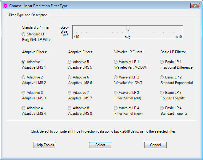
This dialog lists 16 different linear prediction filters that we have been testing. The first 8 are adaptive filters, and the last 8 are earlier designs that have been kept for comparison. The Default Adaptive filter is the first one listed, Adaptive 1. However, you can calculate this filter and any of the others with a different Step Size Coefficient, by adjusting the slider. (For the older filters the slider adjusts a different coefficient.) When you select a filter, it is then calculated and saved as the Alternate filter.
Once you have calculated the Alternate filter, you can compare it to the Default filter by using the Toggle Adaptive Filters toolbar button. This switches between the two filters for an immediate comparison. You can also use the Historical Price Projection to view the Price Projection at any day in the past. For any selected day in the past, you can then click Toggle Adaptive Filters to compare the Alternate filter with the Default filter on that day. (The Splitter Window displays also toggle using these toolbar buttons. Of particular interest is the Adaptive Filter Output display, which shows the whole range of the filter output over the past 1000 days in the form of a graph.) These were all tests that were devised to study the performance of the various filters. Finally, for completeness, you can also calculate the Projected Error Bars using the toolbar button. These are the actual measured error bars, to be compared to the estimated error bars that are shown by default. The estimated error bars, such as shown in the graph above, are obtained by measuring the average absolute deviation (high minus low) over the whole data set, and then extending this forward to future day N by multiplying by the square root of N. (This is just the range predicted by the Random Walk Model.) Then you can toggle between the two types of error bars using the toolbar button. Finally, to go back to the default display, click the Restore Display button.
Standard LP Filter
The original Linear Prediction filter used in QuanTek is the one that I now call the Standard LP filter. This is a "canned" LP filter that is described in the book by Haykin on Adaptive Filters as the Burg Gradient Adaptive Lattice (GAL) filter. This is a very nicely designed filter, for a wide variety of applications, but I finally decided that it was not too well adapted to financial time series. Even though it has some adaptive properties, it seems better suited to situations which are nearly stationary and with a moderate to high signal/noise ratio. A standard example of such a series is the 11-year sunspot cycle, which is nearly, though not exactly, regular and smooth, not noisy. In earlier versions of QuanTek, this filter performed well in some situations and not so well in others. It seems to suffer too much from the syndrome of fitting to the noise (just like the neural network).
When you first open a data file, the Standard LP filter is calculated for the present day only, not all the way into the past. If the Default Adaptive filter has never been calculated, then this Standard LP filter is the only one shown. Once you calculate the Default Adaptive filter, it is shown, but you can still toggle back to the Standard LP filter for the present day. If you want to view the Standard LP filter all the way into the past, you have to calculate it as the Alternate filter using the filter selection at the top of the Choose LP Filter dialog above. Then you can toggle back and forth from the Default Adaptive filter to the Standard LP filter for any day in the past.
Here is the Standard LP filter corresponding to the graph above, obtained by clicking the Toggle Adaptive Filters button:
Notice that the Standard LP filter gives a varying future Price Projection, not just a straight line as in the case of the Default Adaptive filter. The Standard LP filter calculates a set of filter coefficients for the present day, then moves one day ahead at a time and computes a new Price Projection for that day using the same set of filter coefficients. This means that it is using the assumption of stationarity of the time series to extend the Price Projection forward past day 1 in the future. So this is not very realistic, although it is a good strategy for smoother time series with a higher S/N ratio.
In the Short-Term Trading dialog, there is also a display on the right side that uses the 1-day prediction of the Standard LP filter. This may be useful for setting daily buy/sell orders. It lists the 1-day prediction (expected price) of the filter, for the average price (average of high, low, open, close) which seems to be pretty good. Then there is a list box which shows various prices on either side of this predicted average price, together with the percent (of 1-day absolute deviation) deviation away from the predicted average price. In other words, if you click up and down in the list box to the +100% and -100% prices, these are the prices at the expected price range for the day. So this can be a useful tool for setting day buy/sell limit orders at various points in the expected price range, relative to the expected average price. This is one appliction for which the Standard LP filter seems to work pretty well.
References
Harvey, Andrew C.; Forecasting, Structural Time Series Models, and the Kalman Filter; Cambridge (1989)
Haykin, Simon; Neural Networks - A Comprehensive Foundatation; Macmillan (1994)
Percival, Donald B. & Walden, Andrew T.; Wavelet Methods for Time Series Analysis; Cambridge (2000)
Haykin, Simon; Adaptive Filter Theory, 4th ed.; Prentice Hall (2002)
Go back to QuanTek Features