Using the Savitzky-Golay Smoothing Filter

Robert Murray, Ph.D.

Omicron Research Institute

www.omicronrsch.com

(Revised October 19, 2006)

Most technical analysts are very familiar with the ordinary simple moving average (MA) and exponentially weighted moving average (EWMA). These are methods for smoothing the price (or other) series, and various technical indicators such as the MACD can be constructed from them. These methods were devised sometime in the past when the only methods that were available were drawing graphs on graph paper and doing calculations manually. But now that personal computers are available, a much wider range of methods are feasible for constructing technical indicators. This article will describe the Savitzky-Golay smoothing filter, which is a much more sophisticated version of the simple moving average. This filter is widely available as a routine in C, Basic, or other languages, from Numerical Recipes (see references). I have been using the C routine, but perhaps the Basic routine could be incorporated in a VBA program and used with Excel. The book Numerical Recipes also contains an excellent discussion of this and other types of filters and other routines (along with the code itself), upon which the present article is based. (This book also contains many other techniques of Numerical Analysis that would be useful for technical analysts.)

Simple Moving Average (MA)

The simple moving average is the most basic type of smoothing filter. An average is taken over the past N prices, from the current price to the price N-1 days ago, and this average value is taken for the current value of the smoothed price. The number N is the width of the smoothing “window”. This type of filter is called causal because the current value of the smoothed price depends only on current and past prices – no future prices are used. Also, there is an inherent time delay in this type of filter of N/2 days (assuming daily data), which is the delay of the “center of gravity” of the smoothing window relative to the current time. For example, if the price data were a straight line with a given slope, the average value in the smoothing window of this straight line would be its value in the middle of the window. This value is taken as the current value of the smoothed price. But the middle of the window is delayed by N/2 days relative to the current time, so the smoothed price is delayed by N/2 days relative to the current price.

A moving average is used to smooth out the short-time period fluctuations, presumed random, in order to be able to see the longer-term cycles, which are presumed to be the true “signal”. A good discussion of moving averages is in the book by Pring, Technical Analysis Explained. Pring states that, depending on the time period of the cycles you are trying to capture, different window widths N of the moving average are appropriate. This then presumes the existence of discrete cycles in the data, which can be viewed as a deterministic signal buried in the stochastic noise. So the MA can be thought of, from the point of view of Signal Processing, as a de-noising method. This is also discussed in Numerical Recipes. Presumably, the signal corresponds to the lower-frequency, longer-period part of the spectrum, while the higher-frequency, shorter time-period part consists of noise. But the MA is a low-pass filter, which filters out the high-frequency noise, leaving the low-frequency signal. So the smoothed price series from the MA is interpreted as a representation of the signal, consisting of cycles of various long-period components. But the periods of these cyclic signal components are unknown, and the MA with window width N introduces a time lag of N/2 days, which will correspond to an unknown phase shift that depends on the cycle period. This is the trouble with using a causal filter. The unknown phase shift might have a serious effect, unless in the tradition of Technical Analysis it is assumed that there is a long-term trend that is more or less linear and constant, except that it suddenly reverses direction after persisting over a fairly long time. If this were the case, then the phase shift of the MA would be negligible if the window width N is small compared to the time period between trend reversals. But if the period of the signal cycle is not much larger than N, the phase shift will be large compared to the cycle period and hard to estimate.

Savitzky-Golay Smoothing Filter

The Savitzky-Golay (SG) smoothing filter is described in Numerical Recipes. It has a wide variety of configurations, and the simple moving average is obtained as the lowest-order version of the SG filter. This filter can be set to be either causal or acausal (as could the simple MA, for that matter). The N-day window for this filter can be set as in the simple MA to be from the current time to N-1 days in the past, or from the current time to N-1 days in the future, or anything between these values. The acausal filter I prefer has a symmetrical window about the present time, so that using an even value of the window width N, the current time is in the middle of the window. Then the time lag of the smoothing filter will be zero.

According to Numerical Recipes, using the symmetrical window just described, suppose there is a sharp peak in the price data that is being smoothed. Then the moving average window preserves the area under this sharp peak, which is called the zero’th moment. Also, as described above, the position of the peak is preserved, which is called the first moment. But the simple MA smoothing flattens the peak out, so the width of the peak, which is called the second moment, is not preserved. The idea of the Savitzky-Golay smoothing filter is to find a filter that smoothes the data but preserves the higher-order moments, so in particular the widths of features in the data are preserved (along with the positions – no time lag). So the acausal SG smoothing gives a more faithful smoothed representation of the price data than a simple MA.

Polynomial Smoothing

How the Savitzky-Golay smoothing filter works is as follows. Consider again the simple MA filter. In the N-day smoothing window, the value of the smoothing at the right end of the window is taken to be equal to the average of all the price values in the window. In other words, we are taking a least-squares fit of the N prices in the window, to a straight horizontal line or constant value (zero’th order polynomial), and taking the value of the smoothing at the right end of the window to be equal to this constant value. This is equivalent to the zero’th-order SG filter. In the SG smoothing filter, on the other hand, a least-squares fit is made to a higher-order polynomial. A first-order polynomial is a straight line with a constant slope, described by a linear function. This would lead to a first-order SG filter if the data in the window were fit to this straight line. A second-order polynomial is a parabola, described by a quadratic function. This would lead to the second-order SG filter if the data were fit to a parabola. In my applications I have been using the fourth-order SG filter, in which the price data in the window are fit to a fourth-order polynomial. In general, to preserve the widths of narrow features, the filter order should be higher the higher the width N of the smoothing window. But the typical filter orders used are two, four, or maybe six in most cases.

Computing Derivatives

Another feature of the Savitzky-Golay smoothing filter is its capability to compute the derivative of the smoothed price data. From Calculus, the first derivative of a function is its rate of change at a point, or the slope of the tangent line to the function at a point. The second derivative is the derivative of the first derivative, and this measures the curvature of the function at a point. By analogy with Physics, I compute three different acausal smoothings of the (logarithmic) price data. The first I call the Relative Price, which is the smoothed price with an N-day window, minus the smoothing with a 1024-day window. This is similar to a kind of MACD indicator. The second indicator is the first derivative smoothing with an N-day window, which I call the Velocity because velocity is the first time derivative of position. It is the first rate of change of the smoothed price. The third indicator is the second derivative smoothing with an N-day window, which I call the Acceleration because acceleration is the second time derivative of position. It is the second rate of change of the smoothed price. Since the filtering is acausal and there is no time lag, the phase relationships between these three indicators are preserved, and are analogous to the phase relationships that exist between a pure sine wave or cycle and its first and second derivatives. This combination of three indicators I call the Harmonic Oscillator, and I would like to discuss these in greater detail in a separate article.

Any smoothing filter is a low-pass filter, meaning that it passes the low frequencies and suppresses the higher frequencies. With a smoothing window N time units in length, the cutoff frequency of the filter will correspond approximately to cycles with a period twice this long, so that a half wavelength is N units long. So I call the cycle with period (wavelength) 2N the dominant cycle. If a price time series, with daily prices, is filtered by a smoothing filter with window length N, the dominant cycle will be essentially the highest frequency that is passed by the filter, and the smoothed price series will look roughly like a wave with a period of 2N. The three indicators discussed above, the Relative Price, Velocity, and Acceleration, will then each look roughly like waves with period 2N. But the three waves will differ in phase relative to each other. Because it is an acausal filter with no time lag, the Relative Price wave will be in phase with the fluctuations of the price series itself. The Velocity is then one-quarter cycle or 90 degrees ahead of the Relative Price, so it is N/2 time units ahead. This is because when the Relative Price is at a minimum [min], the Velocity or slope of the Relative Price is zero and increasing, or is at an upward moving zero crossing [Z+]. When the Relative Price is crossing zero moving upward, the Velocity is at its positive maximum [max]. When the Relative Price is at a maximum, the Velocity is again zero, but decreasing, so it is at a downward moving zero crossing [Z–]. So it can be seen that the Velocity cycle is 90 degrees or a quarter cycle ahead of the Relative Price. For the same reasons, since the Acceleration is the derivative of the Velocity, it is 90 degrees or a quarter cycle ahead of the Velocity. Keeping track of these phase relationships is obviously important if we want to use these technical indicators to time buy/sell points, especially if the cycle we are timing is the dominant cycle or close to it. An example of this timing problem involving the MACD will be given shortly.

Causal SG Filter

As stated previously, the SG filter can be used for any position of the smoothing window relative to the current time. If the current time lies on the right end of the window, then the SG filter is a causal filter just like the simple MA. In fact, the simple MA in this case is the zero’th-order SG filter. But using the fourth order SG filter, the data in the window are fit by a fourth-order polynomial instead of a zero’th-order polynomial (constant average value). The value of the smoothed data is taken as the value of this polynomial at the right end of the window (current time). But it can be seen that this will drastically reduce the apparent time lag if a fourth-order causal SG filter is used, as opposed to the simple MA. Considering again the example of a straight-line price series, if an SG filter of first order or higher is used, then the fit of this price series to the polynomial inside the smoothing window is exact, so there would be no time lag in this (unrealistic) case. Using the fourth-order SG filter, if the price data were any polynomial up to fourth order, the time lag would likewise be zero, and the smoothing of the price curve would be exactly the same as the price curve itself. For realistic cases, then, the fourth-order causal SG smoothing will have virtually no apparent time lag, compared to simple MA smoothing, so this is a big advantage while still retaining the causal filtering. (However, I prefer the acausal smoothing because it is automatically a zero-phase filter with no time lag at all, so that the phase relationships with the data are preserved.)

Implementing the Savitzky-Golay Smoothing Filter

To use the SG filter, there is a routine in Numerical Recipes that computes the Savitzky-Golay filter coefficients, given the number of data points to the left and right of the current time in the data window, the order of the derivative, and the order of the smoothing (which I take to be four). This routine just computes the filter coefficients – it does not depend on the price data series itself. Then the filter coefficients are utilized in a convolution with the price data to produce the smoothed price data. A separate routine is used for the convolution, which takes as input the price data series of a given length, the SG filter coefficients, and outputs the smoothed price series. This convolution routine uses the Fast Fourier Transform, so the length of the data input must be an integer power of two. This is accomplished by zero-padding the price data, meaning filling up the rest of the array of length n with zeros after the price series. The zero-padding is necessary for the convolution function to avoid the “wrap-around problem”, as described in Numerical Recipes. This can happen when there is not enough zero-padding and the data near the two ends of the data series get mixed together, since the routine treats the data as being periodic. Generally, the minimum number of zeros is of the order of the filter width M, but it does not hurt to use more zeros. Also, I usually de-trend the data by subtracting a line passing through the first and last data points, then add this line back after the smoothing. This eliminates any kind of transients that might occur at the end points, in particular at the present point in time, due to a drastic discontinuity between the price data and zero.

It should be noted again that this convolution routine uses the technique of Fast Fourier Transform (FFT). This means that the smoothing curve can be extended right to the end of the price data series and beyond. This is unlike the situation where the moving average is computed directly. For example, in conventional smoothing with a simple MA of window width N, the first smoothed value would start N days after the first day of prices. If acausal smoothing is used in the conventional smoothing, the smoothed values would begin N/2 days after the first data value, and end N/2 days before the current point in time. But using the convolution routine based on the FFT, the smoothing values can be extended right to the end of the price series and beyond, even for acausal smoothing. This is another nice feature of the SG smoothing filter, compared to conventional smoothing techniques.

Savitzky-Golay Price Projection

When the smoothing is performed, the output of the SG filter actually extends beyond the present point in time into the future, where there was only zero-padding originally. So in this way the SG filter actually produces a Price Projection. This is not the best way to do a price projection – a better way is to use a Linear Prediction filter. However, in a trending market such as in the late ‘90s, this projection would have a certain degree of validity. This is merely a more sophisticated version of the simple method of making a projection from drawing a trend line through the data and extending it into the future, on the presumption that the trend will be continued. This will be valid in a trending market, one that exhibits trend persistence. This type of market is one for which the spectrum of returns is peaked at the low end of the spectrum, corresponding to the constant trend line or the low-frequency cycles. These low-frequency cycles can be regarded as the signal buried in high-frequency noise. So the price is extrapolated by filtering out all frequency components with periods less than 2N, with a smoothing window of length N, and then these low-frequency components are extrapolated by the smoothing filter into the future. These low-frequency components presumably correspond to the signal, while the high-frequency components are the stochastic noise, so what we are doing is using a simple de-noising procedure. This type of procedure is also described in Numerical Recipes.

What I normally do is use the Savitzky-Golay smoothing filter in conjunction with a Linear Prediction filter for the Price Projection. The Linear Prediction filter gives a Price Projection based on correlation in the past price series, and this Price Projection is added on to the end of the past price series to extrapolate into the future. Then the whole series of past plus future projected prices is smoothed using the Savitzky-Golay smoothing filter. By using the smoothing filter on the Price Projection, I hope to filter out the extraneous high-frequency stochastic noise, leaving the lower-frequency modes, which hopefully contain the signal. It should be noted that in the approach described above, where the past price data are de-trended by a trend line passing through the first and last points of the past data, this is equivalent to using a Price Projection consisting simply of a straight trend line with slope equal to the average return, extending from the last price point into the future. Then the past price series and this straight-line future Price Projection are smoothed together with the SG filter, yielding an improved Price Projection.

Incidentally, it should be mentioned here that the other simple type of moving average filter is the exponentially weighted moving average (EWMA). This type of MA is not directly related to the SG smoothing filter, which uses a finite window of length N, while the EWMA uses an infinitely wide (ideally) window. But it has been shown [Durbin & Koopman (2001)] that the EWMA is the Linear Prediction filter for an MA(1) process, a moving average stochastic process of order 1. So this is another example of a smoothing filter that can be used as a Linear Prediction filter. This simple type of prediction filter evidently works well in some situations, those that are well described by the MA(1) process (a special case of an ARMA process). Probably it has been used for the same purpose in Technical Analysis in the past.

MACD Indicator – Phase Shift

The Moving Average Convergence Divergence (MACD), is defined by Pring as a shorter-term EWMA divided by a longer-term EWMA. These are the moving averages of prices, whereas up to now I have been talking about logarithmic prices. If you take the logarithm of the quotient of two prices, this is the difference of the logarithms of the prices. So I use a logarithmic MACD based on log prices, which is the difference of a shorter-term MA minus a longer-term MA. If this indicator is based on the acausal SG smoothing instead of the EWMA, then an example of this kind of MACD indicator would be the Relative Price indicator.

The MACD can be used to time trades. If we idealize the prices as following a definite cycle with some specified period, then we would want to buy at the low points and sell at the high points. These buy/sell points would then be the minima/maxima of the Relative Price indicator defined above, and they would be the positive/negative zero-crossing points of the Velocity indicator. These latter points will always be in phase with the buy/sell points using the acausal SG filter with zero time lag to define the Velocity indicator (at least for past price data). However, the positive/negative zero-crossing points of the MACD indicator are often used as buy/sell points, and this will necessarily involve a certain amount of time lag. If the cycle we are trying to time has a period much longer than the period of the longer EWMA in the MACD, then the MACD acts as a sort of time-delayed Velocity, so these buy/sell points are approximately correct (compared to the long time period of the cycle). However, for shorter period cycles the MACD buy/sell points will be seriously delayed, by an amount that may be hard to determine. This is the problem with using causal MA’s for determining buy/sell points. The buy/sell points determined from an acausal MA with zero time lag, in the past data, will always be in phase (using the Velocity indicator). However, of course, to use the acausal MA to predict future buy/sell points requires the use of some kind of Price Projection, which can itself introduce a phase lag of unknown amount. So neither method is perfect, but at least the zero-lag acausal filter gives the correct buy/sell points in the past data.

Now supposed the cycle period that we are trying to time is much shorter than the longer time period of the MACD. Then if the MACD were constructed using the acausal SG smoothing with no time lag, it would be equivalent to the Relative Price indicator discussed above. We would be timing the buy/sell points according to the positive/negative zero crossings of the Relative Price. But we have already seen that the correct buy/sell points are the positive/negative zero crossings of the Velocity indicator, and the Relative Price lags this indicator by a quarter cycle or 90 degrees of phase. So the buy/sell signals will be too late by this amount if based on the positive/negative going zero crossings of the MACD. If the cycle period is somewhere of the order of the longer time period MA of the MACD, then the phase delay will be somewhere between 0 and 90 degrees, even if constructed using the zero time lag acausal SG smoothing.

If the MACD is constructed using a simple MA or EWMA, there will be an additional time lag in the buy/sell signals of N/2 or N days. The simple MA with window width N has a time lag of N/2. However, if you define the EWMA as exp[-t/N], then it will also have an “effective width” N (equal “areas” of the two windows), but a time lag of N instead of N/2 (from doing a simple integral). So if the length of the cycle we are trying to time is 2N, corresponding to the dominant cycle of the shorter time period MA in the MACD, then the simple MA smoothing will give an additional quarter cycle of phase delay, and the EWMA smoothing will give an additional half cycle phase delay, on top of the quarter cycle due to using the crossing points of the Relative Price instead of the Velocity. If the simple MA is used to time the dominant cycle, this means that the buy/sell signals are 180 degrees out of phase with the correct signals. But we don’t know exactly what the phase delay is, because in the real situation we don’t know the periods of the cycles we are trying to time. The actual price action will be a sum of many cycles, and the actual phase delay cannot be determined.

Phase Correction

The way I have used this type of indicator is to actually measure the correlation of the indicator with future returns, for a given fixed time horizon, and then adjust the phase of the indicator for maximum correlation. In this way any of the various technical indicators based on various types of smoothing could be used to time buy/sell points, once the phase of the indicator is adjusted for maximum correlation with future returns. But if this is not done, there is no way to tell for sure which indicator will give the correct phase relationships, because that depends on the periods of the various cycles we are trying to time. In other words, it depends on the correlation structure of the returns time series. For the past data, the acausal Savitzky-Golay smoothing filter with zero time lag yields a Velocity indicator that is in phase with the returns, but for the future returns there is still an unknown phase shift due to the smoothing of the Price Projection. So to be sure of the correct phase relationships and buy/sell points, this phase shift should be measured and corrected for, by measuring the correlation of the indicator with future returns. The correlation tests that can be used for this are also contained in Numerical Recipes, although it is not hard to make one up from scratch.

Bollinger Bands

One excellent area where the acausal Savitzky-Golay smoothing filter can be used is in the construction of Bollinger Bands. Evidently these are usually based on one or another variety of causal moving average, which means that they will have an inherent time lag. Using the acausal SG filter eliminates this time lag. I like to use the acausal SG smoothing with a window width of 1024 days, in which I plot a center curve and two sets of curves on either side of it, corresponding to one and two standard deviations of the log prices away from the center curve. An example of this is shown here for MSFT stock:

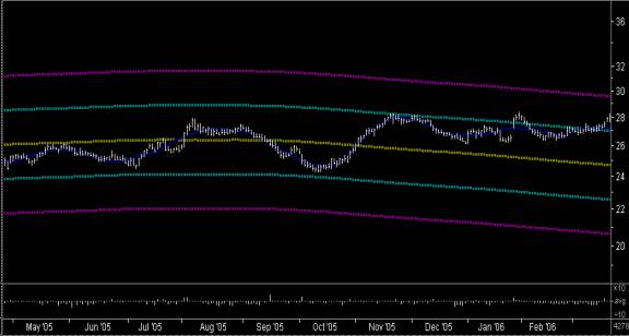
The center curve is dark yellow, the one standard deviation Bollinger Band is dark cyan, and the two standard deviation Bollinger Band is dark magenta. Also, difficult to see underneath the price data, is a dark blue acausal smoothing with a window of 40 days. If you assume a return-to-the-mean mechanism, as we seem to have at the present time for some or most stocks, then the Bollinger Bands can be a useful guide to buy/sell points. The buy points would be between the lower cyan and magenta bands, and the sell points would be between the upper cyan and magenta bands. The price should be within each of these two regions roughly 15% of the time, if Gaussian statistics are assumed to hold (maybe with some “fat tails” in addition). As stated previously, all of these curves can be extended to the present time and beyond, to make a projection, in spite of the long time scale of the smoothing. Normally I use a Linear Prediction filter of some type for the Price Projection, extending the past data into the future, and then smooth the whole time series using the SG filter to obtain the smoothed curves for the Bollinger Bands. But a simple trend line of the type discussed previously could be used instead of the LP filter.

Conclusion

Price smoothing is used in technical analysis because it provides a way to try to de-noise the price data and discern more clearly any underlying signal underneath the noise. A variety of technical indicators can be constructed out of these smoothing curves, for various time scales of smoothing. In previous decades, the simple MA and Exponentially Weighted MA were the main methods for smoothing data, because they were the only methods that were practical to compute by hand. However, now that we have powerful desktop computers, the Savitzky-Golay smoothing filter is practical to use, and it offers a number of advantages over the older methods. The ordinary simple MA is actually the simplest case of the Savitzky-Golay filter, corresponding to the zero’th order filter, but the second and fourth order filters are better because they better preserve the higher moments of the data. The acausal filter also has no time lag, and the causal filter with the higher order smoothing has much less apparent time lag than the zero’th order filter (simple MA). The filter can also compute smoothed derivatives of the data, which offers the potential for an even wider variety of technical indicators to be constructed. The filter can also serve as a simple Linear Prediction filter for the purpose of constructing a Price Projection. However, there are better and more sophisticated methods for Linear Prediction that can be used, and these can be used in conjunction with the Savitzky-Golay smoothing filter. The SG smoothing filter alone is best used for price projection in trending markets that exhibit trend persistence, since the trend is the low-frequency component of the price series, and the SG smoothing filter is just a type of low-pass filter.

References

J. Durbin & S. J. Koopman, Time Series Analysis by State Space Methods,

Oxford University Press (2001)

William H. Press, Saul A. Teukolsky, William T. Vetterling, & Brian P. Flannery,

Numerical Recipes in C, The Art of Scientific Computing, 2^nd ed.,

Cambridge University Press (1992)

Martin J. Pring, Technical Analysis Explained, 3^rd ed.,

McGraw-Hill (1985)

Biography

Robert Murray earned a Ph.D. in theoretical particle physics from UT-Austin in 1994. He obtained a stockbroker license at about the same time, and started his financial software company, Omicron Research Institute, soon afterward. This company is devoted to the study of the Econometrics of the financial markets, and finding optimal trading rules based on Time Series Analysis and Signal Processing techniques. Robert has been intensively studying Time Series Analysis, Signal Processing, and Stochastic Processes since 2001. He has been trading in stocks and studying Technical Analysis since 1988.