Demo: Momentum Indicators - No Smoothing

(Revised October 7, 2006)

In this demonstration, we study the construction of a set of Momentum indicators without the use of the Savitzky-Golay smoothing filter.  To do this, the smoothing time scale is set to zero in the Technical Indicators dialog.  In this way we can work with the raw (log) prices relative to the 512-day smoothing (the dark yellow curve on the Main Graph), or the returns (1st difference of prices), or the rate of change of returns (2nd difference of prices), as technical indicators.  For example, if a minimum of the price at a given time is correlated with positive future returns, then the negative of the past price can be used as a technical indicator (Relative Price).  Likewise, if the past returns are correlated with the future returns, then these past returns can be used as a technical indicator (Velocity), and similarly for the rate of change of returns (Acceleration).  With the zero setting of the smoothing time scale, these first and second differences are computed directly, rather than within the Savitzky-Golay smoothing filter.  In the following we will be studying a representative stock, namely MSFT.

Results of Correlation Test - Filters

We begin by testing the default DWT Linear Prediction filter in the Correlation Test - Filters dialog, accessible from the Hybrid Filter dialog in the Greeting dialog or Main Window.  We select the default settings in this dialog, then run the Correlation Test.  In contrast to some of the other stocks tested, for MSFT the 10-day time horizon does not yield very good results in the Correlation Test.  But a selection of the 20-day time horizon yields good correlation with future returns.  Here is the result of the test for the 20-day time horizon:

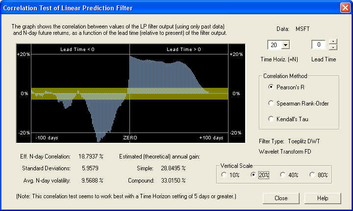
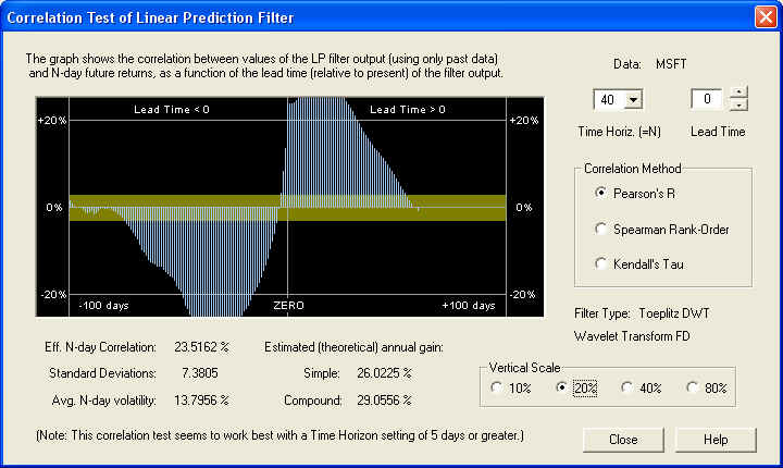
Note the nice positive correlation peak right on the ZERO line, for the Price Projection (returns) due to the LP filter.  Note also the large negative correlation of the past returns with future returns, indicated to the left of the ZERO line.  This possibly explains why the filter performance on the 10-day time horizon is not so good, and also suggest that we can use these past returns as a valid technical indicator.  The 40-day time horizon also yields good results:

By contrast, on the 10-day time horizon, the correlation at the ZERO Lead Time seems to be swamped by the large negative correlation from past returns:

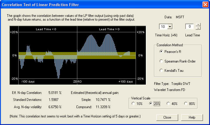
However, please note that the Price Projection further out in the future on this time horizon, shows some good correlation peaks with the future returns in the immediate future.  This is not "cheating" -- the entire Price Projection depends only on past data.  Finally, here is the result on the 1-day time horizon:

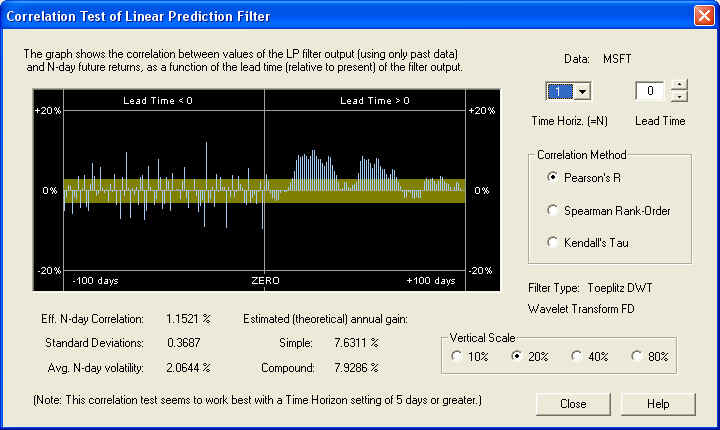
The correlation here is not very good at all, except further out in the future of the Price Projection.  (However, please note the rather distinct negative correlation between the 1-day lagged return (today's) and the 1-day future return (tomorrow's).  Using the negative of today's return as tomorrow's 1-day position should yield an effective short-term trading rule, assuming the correlation persists into the future.)  This shows that on the shorter time horizons, the correlation is masked by stochastic noise.  This noise must be filtered out to display the correlation that exists on the longer time horizons.  In this case, the filtering is done by taking the N-day ordinary moving average (in the Correlation Test), corresponding to the N-day Time Horizon.  In the present situation, it appears that the 20-day time horizon is the optimal choice (or some nearby number).

You can save the 20-day value (the last setting) for the time horizon for the MSFT stock data file when the Close button is clicked to exit the Correlation Test - Filters dialog and return to the Hybrid Filter dialog.  A dialog box appears notifying you that the time horizon has changed, and this value is saved along with the other filter parameters if the Set Filter button is clicked in the Hybrid Filter dialog.  The time horizon for MSFT can also be set within the Correlation Test - Indicators dialog, which is accessible from the Technical Indicators dialog when each individual security data file is open.  In this case, the last setting of the time horizon is saved automatically in the data file when the Correlation Test - Indicators dialog is closed by clicking the Indicators button (but not the Close button), and a dialog box appears notifying you of this.

Estimated Theoretical Annual Gain

Notice that in all of the above dialog boxes, the theoretical estimate for the simple annual gain is given by:

gain = 1.2533 x |Eff. N-day Corr.| x (Avg. N-day Vol.)

The absolute value of the N-day Correlation is to be taken.  Remember that the numbers in the above equation are the percentages from the dialog box divided by 100.  The resulting gain is then multiplied by 100 to get the percentage gain, as shown in the dialog.  The number 1.2533 is the square root of PI/2, which is the factor for converting from average absolute deviation to root-mean-square deviation (for a Gaussian distribution).  (The normalization is 100% average absolute deviation, which corresponds to 100% margin leverage.  But the normalization for the correlation is in terms of r.m.s. deviations.)  The number for the compounded gain is then the simple gain, compounded over 256/N time intervals, where N is the time horizon.

Price Projection as Technical Indicator

Now we open the MSFT data file, by double-clicking on it in the Portfolio dialog bar or using the Open button and selecting it from the Open dialog.  The first thing that must be done is to click Calculate (Stock) Data on the Stock Graph toolbar to calculate 1024 Price Projections, going back 1024 days.  This assumes the data file is at least 2048 days long -- otherwise the result will be compromised.  (Note that this only needs to be done once, as long as the data file is open.)  Once this is finished, click on the Technical Indicators button, the one with the red T in the toolbar.  The Technical Indicators dialog box opens and displays the default settings for the technical indicators, starting with Velocity.  The default setting is the 0-day smoothing time scale for the Savitzky-Golay smoothing filter, which means that the filter is not used at all.  None of the Momentum Ind. buttons are selected, so this default indicator is just a test indicator, not one of the Momentum indicators.

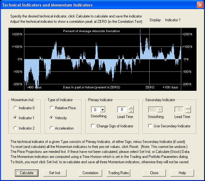
To view the three Momentum indicators that may be saved in the data file, click on each of the three Momentum Ind. radio buttons.  If no indicators are saved, the graph window will be blank.  Or if you want to start off with the default indicators, click the Reset button.  After clicking the Momentun Ind. radio buttons, if you want to reset to the default indicators, click the Trading Rules button, then close the Trading Rules Parameters dialog.  This will display the saved Trading Rules indicator, if any, and clear all the radio buttons.  Then the Reset button will be displayed.  Anyway, select Indicator 1, and the default Velocity indicator shown below.  Then click Calculate to calculate the indicator with the chosen settings.  This indicator is displayed in the graph window:

This setting of the Technical Indicators dialog is special, because in this case the Price Projection itself is the technical indicator.  The (causal) 1-day Price Projection, for each day in the past, is what is shown to the left of the ZERO line.  Exactly underneath the ZERO line is the 1-day Price Projection for the upcoming day.  To the right of the ZERO line is an extrapolation of the indicator using Linear Prediction, but this extrapolation is not really used for anything.  It is the value underneath the ZERO line that is of main interest.  If the Lead Time indicator were set to, say +2 days, then what would be shown under the ZERO line would be the 1-day Price Projection of the return from 2 days in the future to 3 days in the future.  If the Lead Time indicator were set to, say -2 days, then what would be shown would be the past return from -2 days in the past to -1 days in the past.  But since it is set on 0, what is shown is the 1-day Price Projection of the return from 0 days in the future (the present day just ended) to 1 day in the future (the next upcoming day).  Each separate setting of the Lead Time thus corresponds to a separate technical indicator.

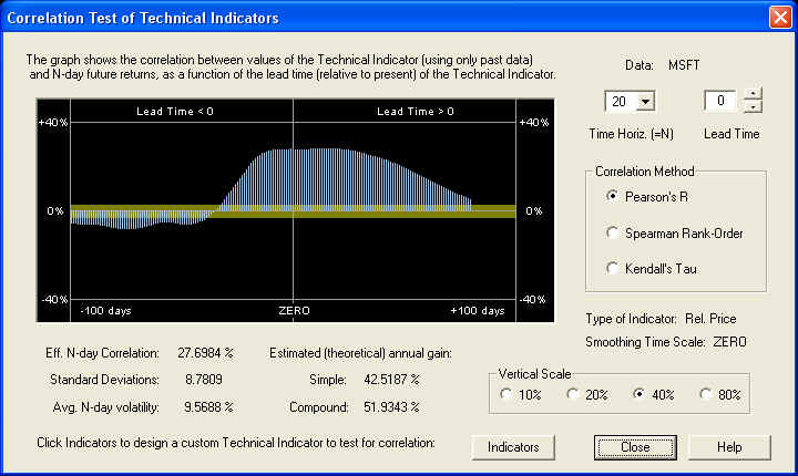
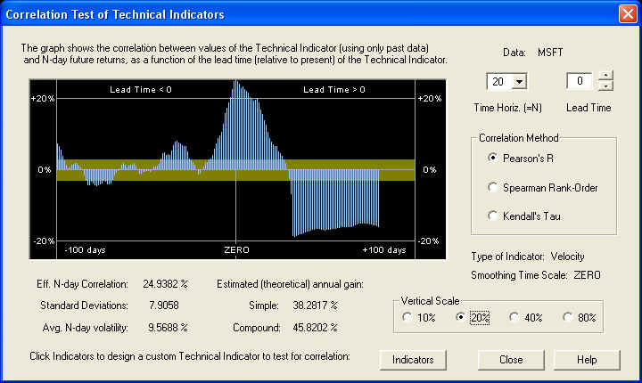
Clicking the Correlation button, we may now view the correlation of the above indicator, for various values of the Lead Time, with future returns.  (The extrapolation to the right of the ZERO line is not used for this, only the values on and to the left of the ZERO line.)  This corresponds to varying the Lead Time setting and plotting the correlation of the resulting technical indicator with future returns as a function of Lead Time.  The correlation value under the ZERO line corresponds to the correlation between the 1-day Price Projection shown above, with future returns.  Actually, this is the case if the Time Horizon is set to 1 day.  Below it is set to 20 days, so what is shown is the correlation between the 20-day Price Projection (average over Lead Time from 1 to 20 days of 1-day Price Projection) and the 20-day future returns:

Please note that the results in this dialog box look exactly the same as the results from the Correlation Test - Filters dialog, on the 20-day time horizon, shown above.  Likewise they are the same for all other Time Horizon settings.  This is because it is the same calculation.  Choosing a zero smoothing time scale for the Savitzky-Golay smoothing filter is the same as no filter at all.  In this case the program simply computes the daily returns, for the past price data together with the Price Projection of the price data, as the technical indicator.  (The Price Projection was computed from the returns in Calculate (Stock) Data, then summed to get the projected prices.)  Then these past and future projected returns, averaged over the 20 day time horizon as a technical indicator, were used in the computation of the correlation of the indicator with the future 20-day returns.  In the calculation done in the Correlation Test - Filters dialog on the other hand, the Price Projection was computed from the returns and the past and projected returns used in the computation of the correlation with future returns.  So you see they are both the same calculation.  We are using the past and projected future returns, averaged over 20 days, as a technical indicator, and it can be seen that this results in some rather nice correlation.  Note also the strong anti-correlation of the immediate past returns with future returns.  This indicates a strong anti-persistence or return to the mean mechanism at work.

Relative Price Momentum Indicator

Next let us go back to the Technical Indicators dialog (by clicking the Indicators button) and see what the Relative Price indicator looks like.  This indicator is just the actual (logarithmic closing) prices and Price Projection from the Main Graph, minus the 512-day acausal smoothing curve of the prices (the yellow curve on the Main Graph), when the Lead Time is set to zero.  Since future returns should be anti-correlated with recent past prices, we go ahead and select the Change Sign of Indicator checkbox.  Then when past prices are down, future returns should be up, and vice-versa (return to the mean mechanism).  We select this for the Momentum Indicator 0 indicator, by clicking the corresponding radio button.  Then click Calculate to compute the indicator and display it in the graph window:

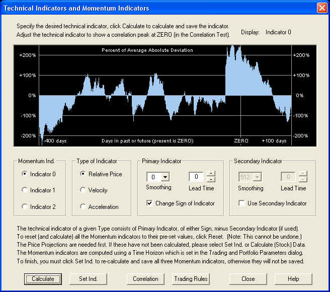
If you look at the Main Graph, there was a sudden drop in price by $3.10, from 4/27/06 to 4/28/06 (Was it a stock dividend?), which explains the sudden discontinuity in the graph of the Relative Price indicator about 40 or so days in the past.  (The Change Sign checkbox is checked, so this shows up as a sudden rise in the indicator.)  Click the Correlation button to show the Correlation Test - Indicators dialog for this indicator:

Note that the scale on this graph is twice the scale of the previous graphs, because the peak correlation is over 20%.  So this shows a very nice anti-correlation between both the past prices and future Price Projection, with future returns on the 20-day time horizon.  Note that we are not having any phase problems now with the Savitzky-Golay smoothing filter out of the picture, as we did in some of the other demos when using this smoothing.  Perhaps this indicates an incompatibility between the Savitzky-Golay smoothing filter and the Linear Prediction filter.  This needs to be investigated further.  At any rate, note the nice, very broad correlation peak, which with the current settings is 8.78 standard deviations away from zero in the Normal distribution.

Velocity Momentum Indicator

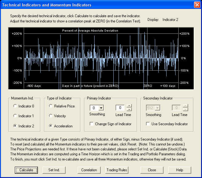
Let us once again go back to the Technical Indicators dialog, by clicking Indicators.  We would like to revisit the Velocity indicator as before.  Using the same settings as before, we click the Calculate button to display the Correlation Test - Indicators dialog.  However, this time, instead of using the positive correlation peak corresponding to the Price Projection, we would like to use the nice negative correlation peak between the past returns and future returns.  Hence we set the Lead Time setting back so that this peak is under the ZERO line, thus:

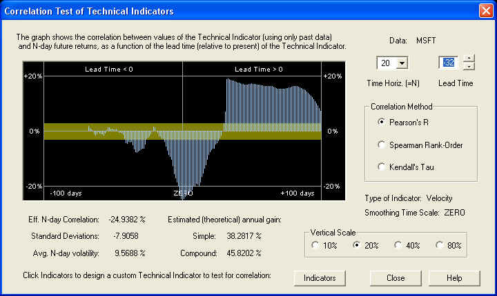
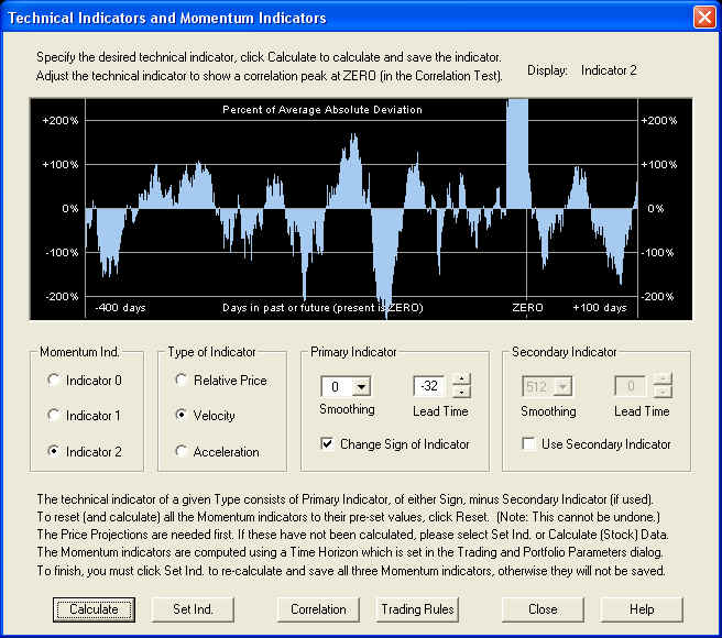
The maximum (negative) correlation occurs when the Lead Time is set to -32 days.  Now go back to Technical Indicators by clicking Indicators.  We can change this to a positive peak by checking the Change Sign of Indicator checkbox.  Then clicking Calculate to re-calculate the indicator, yields a technical indicator consisting of the values of the returns 32 days in the past, averaged over the next 20 days, in the graph window:

Now clicking Correlation to go back to the Correlation Test - Indicators dialog, we can verify that we have a positive peak under the ZERO line:

This correlation graph is just the original one, with the sign inverted, and moved back in time by -32 days.  (Note that the Lead Time setting is now re-set to 0.)  So this setting is also a very nice Momentum indicator.  The correlation with data in the distant past, assumed random, is staying mostly within the one standard deviation band, so this helps verify that this estimate of the standard deviation is not too small.  This provides further evidence that the correlation we are seeing in the above graph is real and not just a statistical fluke.  The large negative peak on the right is, of course, the correlation of the Price Projection (returns) with future returns.  It shows up as a negative correlation because we have the Change Sign of Indicator check box checked.  It is really the past returns that have negative correlation with future returns, but this shows up as a positive peak due to the change of sign.  The Price Projection has a nice positive correlation with future returns.

Acceleration Momentum Indicator

Finally, returning to the Technical Indicators dialog by clicking Indicators, we can check out the Acceleration type of indicator.  We try the following settings, clicking Calculate to compute and display the indicator in the graph window:

Now clicking Correlation to return to the Correlation Test - Indicators, we find the following result:

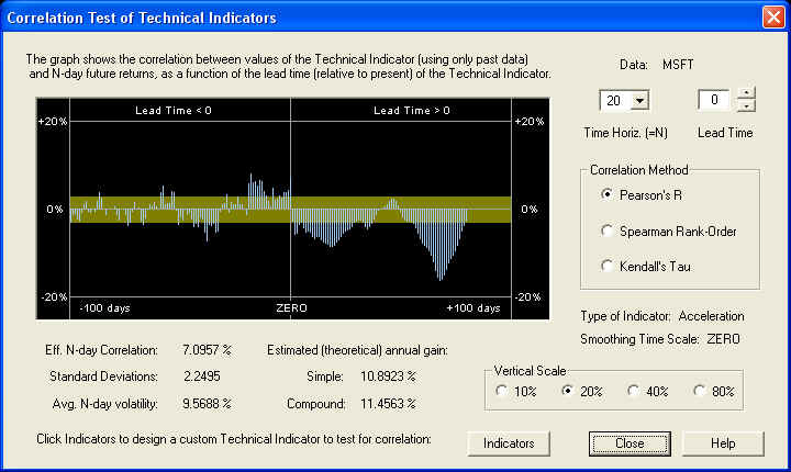
Remember that this indicator is the second difference of the log prices, and does not involve the Savitzky-Golay smoothing filter, since the smoothing time scale was set to zero.  This indicator yields a correlation which is 2.25 standard deviations, so it is probably not random, but it is nothing to write home about either.  So the Acceleration indicator does not work too well for this particular stock.  There is a rather sizable negative peak far out on the Price Projection that we could try to utilize if we wanted, but it would really be better to utilize some other indicator for Indicator 2, instead of an Acceleration indicator.  However, before leaving the Correlation Test - Indicators dialog, once again note that the correlation in the distant past is mostly within the yellow band.  Assuming these are random, this once again confirms that the estimate of one standard deviation of the correlation is approximately correct, and is not too small.  This then confirms that measured correlation of 1 standard deviation has a 68.3% chance of being real, of 2 standard deviations has a 95.4% chance of being real, of 3 standard deviations has a 99.7% chance of being real, and so forth (assuming the random correlation obeys a Gaussian distribution, even though the returns themselves have "fat tails" in their distribution).

Returning to the Technical Indicators dialog by clicking Indicators, we set Indicator 2 to be the same settings as those for the Velocity we had previously, and we set Indicator 1 to be the Price Projection, as it was originally.  Clicking Calculate yields the result:

Clicking the Correlation button, we once again find exactly the same result that we found previously.  So we select this as our third Momentum indicator.  Now select Set Ind. to re-calculate all three indicators and save them in the stock data file.  Then you can close the Technical Indicators dialog.  If you want to view the indicators again, just open this dialog again.  The three indicators are saved in memory for as long as the stock data file is open.  The indicators themselves are also saved in the stock data file, but if you want to calculate the correlations after closing the stock data file, you will have to click Calculate (Stock) Data again to re-calculate all the 1024 Price Projections.

Trading Rules & Diagnostic Test

Finally, with the above settings, and the Price Projection (returns) used for the Momentum 1 indicator, the graphs of the three indicators appear as follows:

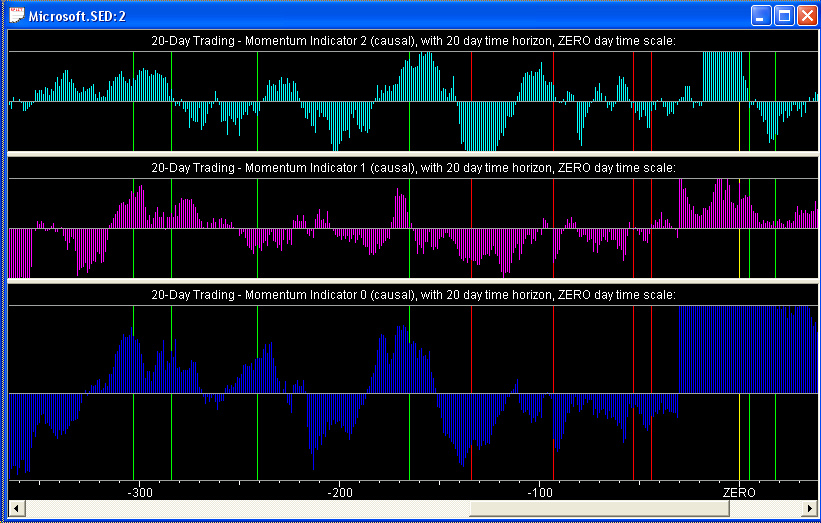
Notice that all three of the Momentum indicators are pretty well correlated with each other, although the correlation is not perfect, of course.  The middle graph, Momentum 1, is the Price Projection itself, and the bottom graph, Momentum 0, is the Relative Price (price relative to the 512-day smoothing curve, with sign reversed).  Both of these are default settings of the Momentum indicators.  The top graph, Momentum 2, is our custom-designed Velocity indicator, with sign reversed, and Lead Time set to -32 days.

Using Future Knowledge

Now, before we examine the results of the Diagnostic Test, a word has to be said about the use of future knowledge in our selection of these three technical indicators.  The Momentum 1 indicator is just the Price Projection (returns) itself.  This Price Projection uses the DWT LP filter with default settings, which seems to give a good result in all cases studied so far.  So no special settings are required for this filter -- the same settings work in all cases.  Likewise, the settings in the Technical Indicators dialog for this indicator are just the default settings, with zero Lead Time.  So this indicator can be regarded as completely generic, and a test of its performance will be a valid test because we made use of no future knowledge in setting the parameters of the indicator.  Likewise, the Momentum 0 indicator also uses the default settings of the LP filter and those in the Technical Indicators dialog, with zero Lead Time.  The correlation in the Correlation Test - Indicators displayed a very nice, broad peak, so this indicator can also be regarded as completely generic.  Both of these indicators are also the default Momentum indicators.  

However, the top indicator, which is a custom Velocity indicator, is different.  We selected a Lead Time of -32 days to bring the correlation peak under the ZERO line in the Correlation Test - Indicators dialog, and we also changed the sign.  In doing so we made use of future knowledge in selecting the value of the Lead Time and the sign of the indicator, based on the historical data over which we are going to test the indicator.  So this indicator cannot be regarded as generic, but instead can only be expected to work for this particular stock in this particular time frame.  However, the rationale here is that the correlation was computed over the past 2048 days (8 years) of data, using 1024 days of data at a time to compute the indicator value 1024 times.  So if this correlation exists over the previous 8 year time interval, it is not unreasonable to expect it to persist up to, say, 100 days further in the future.  In fact, the Momentum indicators need to be re-calculated every day anyway.  So the correlation really only needs to persist one day into the future.  But the time interval over which the indicator settings remain valid should be longer than 1 day, hopefully up to 100 days, and this is a measure of the persistence of the correlation.

The Diagnostic Test is really just a verification, in an actual trading scenario, of the results of the Correlation Test.  If the Correlation Test shows a good positive correlation between the Momentum indicator and future returns, for generic settings of the indicator, then the Correlation Test is a valid test of the predictive powers of the indicator, and so is the Diagnostic Test.  On the other hand, if we need to select special settings of the Momentum indicator to get a good positive correlation, then we have used future knowledge to select these settings.  In that case, the Correlation Test and Diagnostic Test are not valid tests of the predictive powers of the indicator.  But in this case, we fall back on the presumption that if the correlation existed over the past 2048 days of historical data, it should persist some time into the future as well.  So we are relying on the persistence of the correlation, that the indicators selected for maximum correlation with future returns in the past will remain valid at least a short time into the future as well.

Results of the Diagnostic Test

The Diagnostic Test relies only on the saved values of the three Momentum indicators.  So it is not necessary to run Calculate (Stock) Data each time you want to run the Diagnostic Test, so long as the thee Momentum indicators were calculated and saved.  But please note that the results of the Diagnostic Test are a reflection of the correlation found in the Correlation Test - Indicators dialog when designing the Momentum indicators in the Technical Indicators dialog.  So if these indicators are not properly designed, the results of the Diagnostic Test will be poor.

The Diagnostic Test can be run with any mixture of the three Momentum indicators, not just the mixture that is saved with the data file as the Trading Rules indicator.  So we can test each of the three Momentum indicators separately, by setting the corresponding slider to, say, 50% or 100%, and the others to 0%, or we can test any desired mixture of the three.  We will test them separately, and together with all three sliders set to 50%.  We will do this for each of the first four available tests.  These tests are described in the Help file, and the description is repeated here as well:

Trading Rules 0: This is the simplest of the tests, and is designed to measure the effectiveness of the Momentum indicators and Trading Rules directly. These Trading Rules are computed from closing price data, so for the sake of this test the buy and sell points are also taken to be at the closing price. In other words, it is assumed that, just before the close, the latest price data are downloaded, the QuanTek program is run, the Trading Rules and optimum position computed, then the position is adjusted at the closing price for the current day. The position is held until the closing price for the next day, then the new position is established at that time. In other words, this test measures the effectiveness of the Trading Rules in 1-day trading, from the current day's close to the next day's closing price.

Trading Rules 1: This test is similar to the previous one, except that the position is established at the opening price for the next day and the position is closed out at the closing price for the next day. The results for this test are generally not as good as for the previous test, indicating that important price movements are likely to happen after hours in overnight trading, so it is a good idea to maintain a position from one trading day to the next.

Trading Rules 2: This test is established at the opening price and closed out at the closing price. In this test, instead of establishing a position proportional to the Trading Rules, a simplified rule is used: If the value of the Trading Rules is between -50% and +50%, the trading position is zero. If the Trading Rules are greater than +50%, the position is established at +100%, and if the Trading Rules are less than -50%, the position is established at -100%.  Relative to the amount of equity invested, this rule may give better results than when the position is proportional to the Trading Rules, and it is much simpler to implement.

Trading Rules 3: This test is similar to the previous one, being established at the opening price and closed out at the closing price. However, if the Trading Rules are greater than 0%, the position is established at +100%, and if the Trading Rules are less than 0%, the position is established at -100%.  The results from this method do not seem to be as good as the previous method, relative to the equity invested, because the amount invested is always 100%, whether long or short, regardless of the prospects for a move in prices.

The fifth test is just random numbers, and the sixth test consists of holding the equity constant as the price varies.  This last test gives a small, but consistent, gain, but we will not run this test.  The random numbers test is a good way to gauge the standard deviation of the gains, since a different set of random numbers is generated for each run.  (The mean trading gain from random numbers should, of course, be zero.)

Each Momentum indicator is normalized to 100% average absolute deviation (margin).  In the Trading Rules, these three Momentum indicators are added together after multiplying by the slider setting, and dividing by two.  Thus if they were in perfect sync, with each slider set to 50%, then the average absolute deviation of the Trading Rules should be 75%.  However, since they are not in perfect sync, the average absolute deviation will be more like 50% if the indicators are designed properly and all three sliders are set to 50%.  So for the Trading Rules 2 test to work properly, the sliders should be set to 50%, which is what was done for test TR 2.  If that is the case, then there should be a long or short position roughly half the time, and zero the other half.  To test the trading rules for a different threshold, set the slider bars to different values for this test.

The results of the Diagnostic Test are expressed in terms of simple annual gain, corrected for 100% margin.  For comparison with the results of the Correlation Test given above, we note here the estimated (theoretical) simple annual gain, from the dialog boxes shown previously, for each of the three indicators:

Momentum 0: 42.52%        Momentum 1: 28.85%        Momentum 2: 38.28%

Test	Mom. 0	Mom. 1	Mom. 2	Mix.
TR 0	32.17%	24.21%	33.58%	34.11%
TR 1	24.58%	23.72%	26.39%	28.37%
TR 2	52.10%	-9.62%	74.74%	23.52%
TR 3	24.55%	5.96%	21.98%	32.02%

By contrast, the Buy & Hold return was -3.84% over the time interval.  Considering the rather large statistical variance of the results of active trading, the measured gains agree rather well with the estimated gains.  In the TR 2 test, the margin leverage was only around 5% to 10% or so, so a rather wide statistical variance in the gain can be expected.  The trouble with such a trading strategy as TR 2 is that it greatly increases variance of returns, or risk.  All the results are more or less as expected, except for the last two tests using the Momentum 1 indicator, which is just the Price Projection (returns).  However, this indicator performs well on the first two tests.  But the equal mixture of all three Momentum indicators, making up the Trading Rules indicator (in this case), performs very well on all four tests, as do both the Momentum 0 and Momentum 2 indicators.

Of course, these are only simulated results.  Although every effort has been made to make this a valid and fair test of the predictive capability of the Momentum indicators, there is no way to say with certainty that no future knowledge has crept in somewhere.  The Diagnostic Test is only an estimate or simulation of various trading scenarios, not the real thing.  QuanTek makes use only of past price data to derive the Price Projection and Trading Rules, not fundamental or economic data.  In real-life trading or investing, the trader or investor must make use of all available information in formulating trading and investing decisions.

return to Demonstrations page