Making a Price Projection Using Linear Prediction Filters
by
Robert Murray, Ph.D.
Omicron Research Institute
www.omicronrsch.com
(Revised September 28, 2006)
It has been widely believed for the past century or so that financial returns follow a Random Walk [Bachelier (1900)]. There is still a lot of controversy about this. However, it seems increasingly clear that the characterization of financial returns series as a Random Walk is a good approximation, but the true situation is far more complex. A Random Walk (or “Brownian Motion”) is an example of a stochastic process; in fact it is the simplest form of stationary stochastic process. In the Random Walk model, the (logarithmic) price returns – differences of the logarithmic price from one close to the next, say – are modeled as independent Gaussian random variables with a constant mean and variance. The constant mean and variance is what characterizes the process as stationary. The constant mean of the returns implies that there is a constant linear trend (in the log prices), and the constant variance of the returns implies that the volatility is constant with time. The fact that the returns are independent random variables means that they are uncorrelated. So this is a very simple type of stochastic process, but it is “too good to be true”. If the Random Walk model held, with a non-zero, constant trend in the prices, then the only sensible trading strategy would be the “Buy & Hold” strategy, corresponding to this constant linear trend. (The expectation value of the gain from active trading would be zero.) Unfortunately, the true stochastic process of the returns sequence is a far more complex, nonstationary, time series. The Random Walk model is too simplistic.
If the Random Walk model held, then markets would be efficient, and future prices could not be predicted from any knowledge of past prices (or any other past information). But the whole objective of Technical Analysis is precisely to find functions of the past price history which yield information as to future price moves. Another way of saying this is that technical indicators are functions of the past returns, which are correlated with future returns, over some time horizon. Even though the markets are very efficient and the returns series is approximately a Random Walk, at least at first glance, even a very small inefficiency and very small correlation of past returns with future returns would be enough to yield substantial profits from active trading. This makes it worthwhile to search for this small correlation between functions of the past returns and future returns. In the process we can learn more about the exact nature of the nonstationary stochastic process that describes the financial markets. An early pioneer in this direction was Benoit Mandelbrot [Mandelbrot & Hudson (2004)], who incidentally was the mathematician who first “discovered” the concept of fractals. The fractal concept is related to certain types of stochastic processes, known as “long-memory” processes, that are thought to describe financial time series, as described by Edgar Peters [Peters (1991, 1994)]. These processes are characterized by a parameter that Peters calls the “fractional difference parameter”, but I like to call the fractal dimension (even though this is not strictly correct – it is shorter).
So the problem is to find functions of past returns, called technical indicators, which are correlated with future returns. We can try to construct various functions of this sort, to give an indication of when to buy and sell in active trading. An example of this is the nonlinear function of past returns used by Rick Martinelli in his recent article (June 2006). However, another related approach is to use filter theory to derive a Linear Prediction filter, which is an algorithm to find an optimal linear function of past returns which yields the best estimate of the future returns themselves, based on correlation in the past data. The standard filter theory assumes the stochastic process is stationary, although this cannot be strictly true. However, over a certain period of time, such as 1024 trading days, it might be a reasonable approximation. Or, if it is believed that short-term, time varying correlation is present, then the filter can be computed over this shorter time interval using the stationarity assumption, but updated every day, thereby taking into account the nonstationarity. (This is what would be called an adaptive filter.) Martinelli emphasizes a very short-term range of data of only 3 days, while I emphasize the long-term correlation over the 1024 day (4 year) time period.
Another view of Technical Analysis is that it is an attempt to solve the “de-noising” problem of financial time series. The Random Walk model states that financial returns are just uncorrelated “white noise”. However, most of us believe that there is an underlying “signal” buried deep within all the “noise”, and if we knew the true signal then we would know how to time our trades for maximum profit. If the signal is thought of as the real price moves which are in response to previous price moves and various external factors, and if we can separate this underlying signal from the noise, then there is the possibility of formulating trading rules to take advantage of the future price moves. So one way to view Technical Analysis is that it is an attempt to “estimate” this true signal buried under the noise, in which case the signal constitutes the returns, and we are attempting to estimate the future values of the signal, or returns, from their past values. The technical indicator is thus our best estimate of the “signal” buried underneath the “noise”. However, this signal estimation is also the purpose of a Linear Prediction filter, to give an optimal prediction of the future signal, based on measured correlation in the past data (or an optimal estimate of the past signal, in the case of optimal smoothing).
Linear Prediction Filters
I have been experimenting with various types of Linear Prediction filters using my QuanTek program, which also contains a variety of statistical tests of the returns data. A couple of the most important tests are two different ways of computing the spectrum of the data, which are the Periodogram spectrum and the Wavelet spectrum. The Periodogram spectrum is based on the Fast Fourier Transform (FFT), while the Wavelet spectrum is based on the Discrete Wavelet Transform (DWT). Using the Wavelet spectrum it is possible to see graphically the existence of a nonzero fractal dimension, thereby signaling the presence of a “long-memory” process (if the fractal dimension is 0<d<+0.5) or an “intermediate-memory” process (if the fractal dimension is –0.5<d<0). The fractal dimension of 0<d<+0.5 corresponds to trend persistence, while the fractal dimension of –0.5<d<0 corresponds to trend anti-persistence. It should be noted that normally in Technical Analysis, only the trend persistence case is assumed to hold. However, from the results of the measurement of the DWT spectrum on a variety of stocks, it appears that the current market conditions may be characterized by trend anti-persistence, for the most part. This may also be thought of as a return to the mean mechanism of stock prices.
The Linear Prediction filters I have been experimenting with are themselves based directly on the Periodogram spectrum or Wavelet spectrum. This is because the spectrum of the returns series is directly related to the autocorrelation sequence of the series. If the returns are uncorrelated, as in the Random Walk model, then each return is (perfectly) correlated with itself and the correlation with all the other returns is zero. Then by a theorem called the Wiener-Khintchin theorem [Numerical Recipes (1992)], the power spectrum is the Fourier Transform of the autocorrelation sequence. This means that in the Random Walk model, where the correlation between returns is zero, the power spectrum will just be a constant for all frequencies – a completely flat spectrum. This is why this spectrum is also known as “white noise”. So by looking at the spectrum, we can tell if there is any correlation between returns, from the deviation of the spectrum from a constant, white noise spectrum. However, there is a major problem, which is that the true spectrum itself (in the stationary approximation) is buried in stochastic noise. So if you look at the Periodogram for a sequence of Gaussian random variables, it will not look flat, but instead will look completely jagged and random. So the big problem is how to find any “signal” or true correlation that might exist, buried underneath all this stochastic noise in the spectrum or the returns series. Finding this hidden signal is what Technical Analysis is all about, as well as the theory of Linear Prediction filters. This is called the estimation problem for the LP filter, and there are different approaches to solving it. It is, however, a difficult problem. (And according to the Random Walk theory of the market, it is impossible.)
I have experimented with several different ways of computing or estimating the Linear Prediction filter. The most promising approach so far is based on the Wavelet spectrum. This is the best way for estimating the fractal dimension of the process, since the low-frequency end of the spectrum is emphasized in the Wavelet approach, and this approach is a very natural one for modeling long-memory or intermediate-memory processes. The Wavelet power spectrum is computed by taking the DWT transform of the returns and squaring it to get the power spectrum. The wavelet decomposition works by dividing the returns series into wavelet coefficients that depend on both frequency octaves and on time. The time dependence is then averaged over to get just the spectral power in each frequency octave. Then this Wavelet spectrum is used to estimate the autocorrelation sequence, by Fourier transforming it, and from this the filter coeffients are computed by means of a standard method (Wiener-Hopf equations). This averaging process is really a method of “de-noising” the power spectrum, and I am getting consistently good measurements of correlation between the filter output and future returns using the Wavelet-based Linear Prediction filter. Another approach is the one based on the Periodogram spectrum, which leads to a standard ARFIMA filter [Peters (1994)]. In this approach I still use the Wavelet spectrum to (try to) estimate the fractal dimension, but I separately use the Periodogram spectrum. The fractal dimension must actually be set manually in this approach. The Periodogram is smoothed by a method, which is essentially the same as limiting the length of the filter coefficients to a set of N coefficients. I call this the Order of Approximation. This determines the approximation of the time series by an ordinary AR(N) process. On top of this, I multiply the response by that of a fractional difference filter with the fractal dimension which must be set “by hand”. This gives the “fractionally integrated (FI)” part of the ARFIMA filter. (There isn’t any “moving average” or MA part – it is really just ARFI.) This approach gives good results for the “fractionally integrated” or fractional difference part of the filter, provided the sign of the fractional difference parameter or fractal dimension, is estimated (or guessed) correctly beforehand. However, the estimation of the parameters for the AR part of the filter is usually not too good. This is what leads me to believe that most of the “signal” resides in the low-frequency components of the spectrum, and the high-frequency components are mostly stochastic noise. At least this is the case for linear functions of the returns, or maybe it is due to the assumption of a stationary process inherent in the Fourier methods. At the present time I am not seeing much evidence at all of any trend persistence in the data. Most stocks seem to be displaying a negative fractal dimension, which indicates trend anti-persistence. So market conditions seem to be completely different from those of the late 90’s, which is another indication of the non-stationary aspect of the market returns series.
The Wavelet filter works very well on its own, with the same default settings all the time. It is able to estimate the fractional difference parameter or fractal dimension (implicitly, through the Wavelet spectrum) and correctly take into account the “long-memory” or “intermediate-memory” behavior of the returns series. So, the results of the correlation test are a fair test of the predictive powers of this filter. This filter is indeed able to find the “signal” buried in the “noise”, due to the Wavelet decomposition of the returns series. The filter based on Fourier techniques, on the other hand, suffers from the defect that the fractional difference parameter or fractal dimension must be set “by hand”. It is crucial to get the correct sign of this parameter; otherwise the prediction of the filter will be anti-correlated with future returns, not correlated, as we would wish. But the estimation of the fractional difference parameter relies on an analysis of the data we are trying to predict, or in other words, on future knowledge. So in this sense, the test of this filter is not quite “fair”, in that the results are based on the correct knowledge beforehand of the sign of the fractional difference parameter. This is a major defect of the Fourier-based Linear Prediction filter, but since it is a standard method for time series analysis, it is interesting to study for purposes of comparison of techniques. However, for financial time series, which are almost certainly non-stationary, we prefer to place our faith in the Wavelet techniques.
Wavelet Spectrum and Periodogram Spectrum
Here is a very nice example of a stock whose returns display a significant negative fractal dimension. In the top display is shown the actual measured DWT spectrum, while in the bottom display is shown the spectrum corresponding to a pure fractionally integrated process with fractal dimension equal to –0.16. This spectrum is obtained by specifying the FFT filter, with Order of Approximation of zero and Fractal Dimension setting of –16, denoting the value –0.16. (Note that only the lower frequency half of each spectrum is displayed in the graphs.):
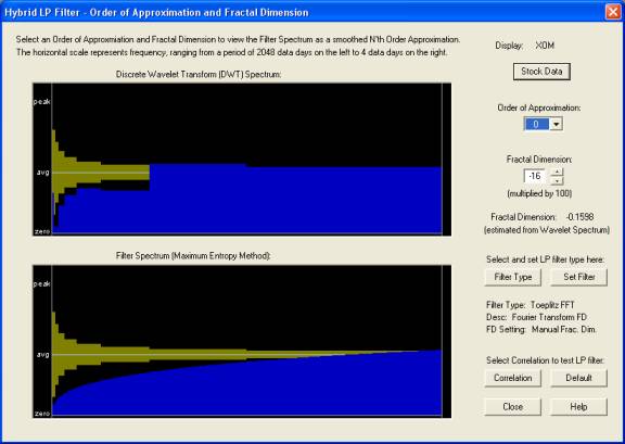
Notice how the spectrum rolls off fairly smoothly at low frequencies in the actual spectrum in the top display, which is approximated pretty well by the spectrum of the “intermediate-memory” process in the bottom display. (The approximate one standard-error bars for each frequency octave of the DWT spectrum are show in dark yellow.) The bottom display shows the spectrum derived from the FFT filter coefficients with the settings shown, by the so-called Maximum Entropy Method [Numerical Recipes (1992)]. However, the Wavelet (DWT) filter uses the spectrum exactly as shown in the top display, with no need to set the fractal dimension by hand, so for these reasons I view it as a better approach. But to display the spectrum of representative ARFIMA filters in the bottom display, the FFT filter settings can be used. (Note that this spectrum uses 2048 days, or 8 years, worth of data, assumed stationary over this time interval.)
By contrast, here is the Periodogram spectrum for the same stock:
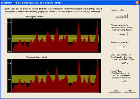
From the standard theory of the Periodogram [Brockwell & Davis (1991)], it is necessary to smooth the Periodogram in order to reduce the standard deviation of the result. The above is smoothed over a 6-day period, but this smoothing can be selected over a wide range. Also, the result can be compared with the spectrum of a series of Gaussian random variables. In the above spectrum, it is much harder to see the roll-off at low frequencies, which is (evidently) the most important part of the “signal”. The other peaks and valleys are (I think) just random noise, although the Kolmogorov-Smirnov test indicates a 98.79% probability that this spectrum is that of a non-random returns series. (It is non-random to the 1.21% significance level.) Note: The bottom display shows an alternative (standard) method of computing the spectrum, which is derived from the coefficients of a standard Linear Prediction filter computed from the Levinson-Durbin (or Burg) method, using again the Maximum Entropy Method [Numerical Recipes (1992)]. It is because of the random noise in the Periodogram and the inherent assumption of a stationary time series that the Fourier methods are not so good for financial time series. They are more suited to situations like electronic signals, where everything is periodic and the statistics do not change with time.
Correlation of Linear Prediction with Future Returns
So the important and non-trivial problem is how to separate the “signal” from the “noise” in financial time series. This is the main crux of the matter. The effectiveness with which this is done can be measured by measuring the correlation between the output of the Linear Prediction filter, or the technical indicator, and future returns, over some time horizon for trading. We are finding that for short time horizons, for example 1 day, the correlation is usually masked by stochastic noise and is usually not evident. But by taking longer time horizons, most of the stochastic noise can be averaged out, and then some non-trivial correlations emerge between the longer-term Price Projection, or longer-term smoothings of the technical indicators, and the longer-term future returns. (It could be that the shorter-term correlations are being averaged over because of the stationarity assumption.) Here is a display of the correlation between the past returns and future Price Projection (returns), with the future returns, for the same stock as before:
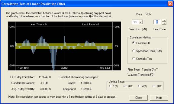
The way this display works is as follows. The Time Horizon is set for 10 days. Therefore, the correlation of the 10-day forward average of returns, for each day in the past, and for each day of the future Price Projection (returns) is computed with the 10-day forward average of the actual future returns. This past and future correlation is displayed on the graph, with number of days in the past or future indicated on the horizontal axis. The correlation under the ZERO line means the correlation between the immediate 10-day forward average of the Price Projection (returns) and the 10-day forward average of the future returns. It can be seen that there is a nice positive peak under this line and extending several days into the future of the Price Projection. However, also noteworthy is the very large negative correlation peak about 22 days in the past, between these past returns and future returns. This negative correlation goes along with the negative fractal dimension noted earlier, and is indicative of anti-persistence or a return to the mean mechanism. So a very effective technical indicator could be constructed by taking a 10-day simple moving average, from 22 days in the past to 11 days in the past (inclusive), and using (the negative of) this as an indicator of the future trading position, to be held for the next 10 days. This technical indicator would not even depend on the output of the Linear Prediction filter at all. But this indicator would be likely to work only in the current market environment, with those stocks that display a negative fractal dimension. In fact, it can only really be applied to this particular stock, in this particular time frame. In other markets, such as the trending market of the late 90’s, an indicator based on trend persistence rather than anti-persistence would be called for (for most stocks).
Price Projection
The actual Price Projection from the Wavelet LP filter is perhaps the most important technical indicator of all in the QuanTek program. This Price Projection can be used to estimate the expected return over time horizons ranging from 1 to 100 days, for the purpose of trading or portfolio optimization. The Price Projection for a stock like XOM does not look very exciting, because we have already established that the stock is exhibiting a return to the mean mechanism, so its Price Projection will be more or less “flat”. However, this is just as well, because we want an estimate of the returns that excludes the stochastic noise as much as possible. Here is the Price Projection for XOM stock, using the DWT Wavelet filter (in blue):
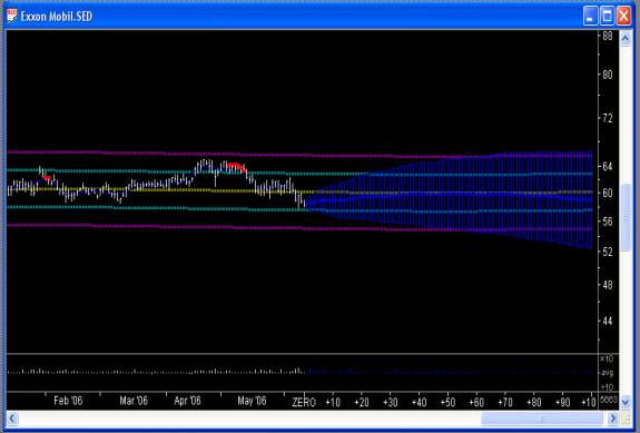
It can be seen that this Price Projection does have some structure, even for a large, heavily traded company like XOM. For a smaller, more volatile and more thinly traded company, the correlation in the past returns will be greater, and the Price Projection will show correspondingly more structure. Also the “return to the mean” mechanism is clearly visible in this Price Projection, corresponding to the negative “fractal dimension”. Then due to the correlation test just described, we can be assured that this Price Projection has at least some validity as a prediction of future price action. Of course this is only an estimate – it is impossible to take into account all the factors affecting stock price and make a deterministic prediction of future price moves. Stock prices move according to a stochastic process.
Future Plans
This Wavelet filter is based on the assumption of stationarity, because the Wavelet spectrum has been averaged over time in each frequency octave. However, the wavelet approach is very well suited to describing nonstationary time series as well, since the wavelet basis retains a time dependence in each octave. I are currently working on such a version of the Wavelet filter, in which the spectrum is not time averaged. But the filter will make use only of the DWT components in the most recent past, because the ones in the distant past will not affect the present. Each frequency octave of the spectrum should control the Price Projection out to a number of days N, where N is the period corresponding to each frequency octave. So the shorter-term projection should be more volatile, since it is based on more high-frequency DWT components, and it will smooth out further into the future on the Price Projection, as only the lowest-frequency DWT components have an effect. It is for this reason that the Wavelet approach is well suited for many types of time series appearing in practice, while the Fourier approach is really only suited to time series that are known to be periodic over a long period of time, such as might be encountered in electronic circuits for example. Another approach is that of the Kalman filter. The Kalman filter is basically a method for the recursive calculation of a smoothing or prediction, using only past data, leading to a causal indicator or Price Projection. However, the essential problem in Technical Analysis is really the de-noising problem and signal estimation, which is best done using Wavelet methods, and at present it is not at all clear how to combine the Wavelet methodology with that of the Kalman filter. The Wavelet methods do not seem to lend themselves very readily to a recursive calculation using a Kalman filter (although I may change my mind about this later).
References
Louis Bachelier, “Théorie de la Spéctulation”,
Anneles de l’Ecole Normale Superiure (1900)
Peter J. Brockwell & Richard A. Davis,
Time Series: Theory and Methods, 2nd ed.,
Springer-Verlag (1991)
Ramazan Gencay, Faruk Selcuk, & Brandon Whitcher,
An Introduction to Wavelets and Other Filtering Methods in Finance and Economics,
Academic Press (2002)
Benoit Mandelbrot & Richard Hudson, The (Mis)Behavior of Markets,
Basic Books (2004)
Rick Martinelli, “Harnessing The (Mis)Behavior of Markets”,
Technical Analysis of Stocks & Commodities, June 2006, p.21
Donald B. Percival & Andrew T. Walden,
Wavelet Methods for Time Series Analysis,
Cambridge University Press (2000)
Edgar E. Peters, Chaos and Order in the Capital Markets,
John Wiley & Sons (1991)
Edgar E. Peters, Fractal Market Analysis,
John Wiley & Sons (1994)
William H. Press, Saul A. Teukolsky, William T. Vetterling, & Brian P. Flannery,
Numerical Recipes in C, The Art of Scientific Computing, 2nd ed.,
Cambridge University Press (1992)
Biography
Robert Murray earned a Ph.D. in theoretical particle physics from UT-Austin in 1994. He obtained a stockbroker license at about the same time, and started his software company, Omicron Research Institute, soon afterward. The QuanTek Econometrics program started out as StockEval, a Technical Analysis and stock-trading program, which featured the Price Projection, based on a standard Linear Prediction filter. The current QuanTek program uses the same basic technique, but is supplemented by a variety of statistical tests of market returns data, as well as the capability of designing a set of custom, causal indicators and testing these for effectiveness using the correlation tests in the program. This program makes use of established principles of Econometrics and Time Series Analysis to as great a degree as possible. Robert has been intensively studying Time Series Analysis and Signal Processing since 2001. He has been trading in stocks and studying Technical Analysis since 1988.