Demo: Fractional Difference Filter
(Revised May 28, 2005)
This demonstration is an experiment to test the Fractional Difference filter used by QuanTek. This filter is called by them the "best linear predictor of the fractionally integrated noise process" [Brockwell & Davis (1991)]. This fractionally integrated noise process is in turn described by a difference equation with a fractional exponent, hence the name. The hallmark of a fractionally integrated noise process (ARIMA, or Auto-Regressive Integrated Moving Average process, fractionally integrated) is that the autocorrelations decay like a power law, rather than exponentially as in the case of a normal ARMA process. Hence these processes are also called "long memory" processes.
It has been argued by Edgar Peters in his book, that stock returns are described by a long memory process with a positive fractional dimension parameter. This would confirm the long-term trend persistence of stock data. This indeed seems to be true for very long time horizons. However, we are finding that over the short to intermediate term, such as a 1-day to 40-day time horizons, the Fractional Difference filter gives superb results (for MSFT stock over a recent 1024-day time interval) using a negative fractional dimension parameter. This seems to be due to the fact that, for short-term to intermediate-term returns, the trend is anti-persistent, indicating a return to the mean mechanism. In other words, there is a pronounced anti-correlation of daily returns over these time periods. Evidently the Fractional Difference filter with negative fractional dimension parameter is just picking up this anti-persistence and anti-correlation in the short-term returns data.
Example: MSFT Stock
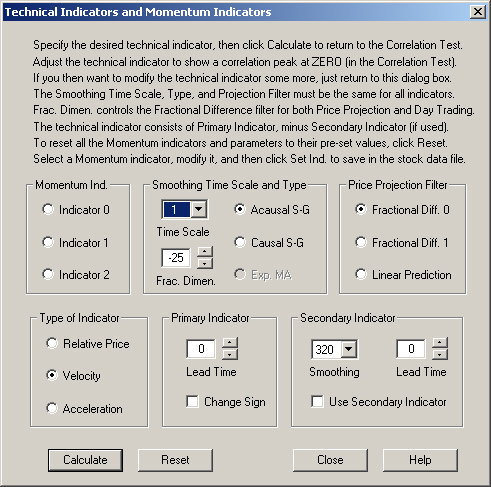
We first compute a Technical Indicator using this filter. This indicator consists of a function of the past stock data, indexed by the time index. In the present case, the function for the past values of index are just the past returns ("velocity"). The function for future values of the index are just the output of the Fractional Difference filter, extrapolated out to 100 days in the future. The Smoothing filter is not used, so the Smoothing Time Scale is set to 1 day. The value of the fractional dimension is set to -25. The settings for this technical indicator are given here:
The result of computing the correlation between the values of this technical indicator as a function of its time index, and the 1-day future return, is given as follows. This result is for a 1-day time horizon:
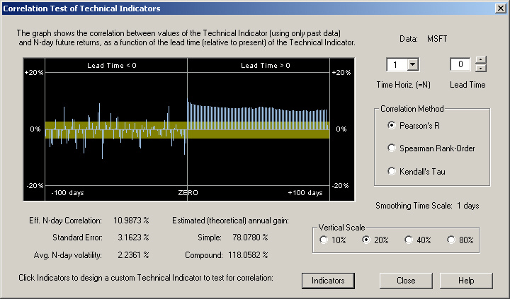
According to the definition of this technical indicator described above, the values of correlation to the left of the ZERO line are just the autocorrelations of the past returns with the 1-day future return. Notice in particular that for the past 5 days these autocorrelations are negative. This seems to be the case almost all the time for most stocks. Due to the way the output of the Fractional Difference filter is extrapolated ahead, there is a positive correlation between this output and the 1-day future return, all the way out to +100 days. However, the correlation is greatest at Day 1. It can be seen that this correlation is nearly 11%, which yields an estimated theoretical simple gain of more than 78%! This is really phenomenal, and proves that correlation exists in the short-term returns after all!
For a 20-day time horizon, the 20-day average of the values of the technical indicator over the next 20 days, starting at the given index, is correlated with the 20-day return. The result of this is shown here:
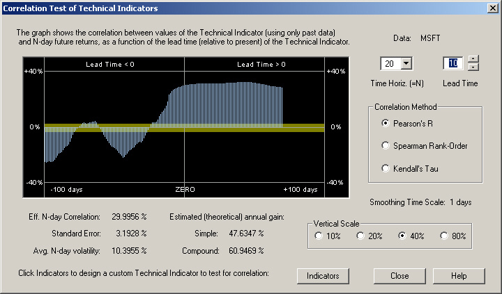
It can be seen that the Fractional Difference filter still gives superb results over this time horizon. However, in this case the trading rules are more optimum when a 10-day Lead Time is used.
We see more or less the same result with a 40-day time horizon:
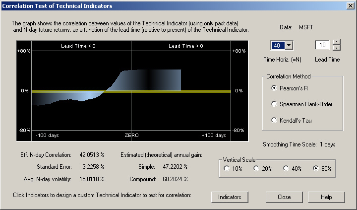
In this case, the Lead Time is still set for 10 days.
To verify the above correlation and estimated theoretical returns, the Diagnostic Test was run using the Fractal Difference filter in Day-Trading. There are two different Day-Trading tests to choose from in the Diagnostic Test. These are called the Day Trading-Fixed and Day Trading-Float tests. The Day Trading-Fixed test is the one closest to the computed correlation and estimated theoretical gain in the Correlation Test dialog. The Day Trading-Float test makes use of the opening price each morning to adjust the recommended position.
In the Day Trading-Fixed test, the trading rules are computed from the close price at the end of the day to the close price the next day. It is presumed that a trader can wait until, say, 5 minutes before the close, download stock data, run the QuanTek program, get the computed estimated 1-day return, then buy or sell at the close price. (Buying or selling at the close is not unheard of as a practical trading strategy.) The results of the Diagnostic Test for the Day Trading-Fixed test are given as follows:
The average absolute daily position (margin) as a percentage of the (constant) equity is: 53.97 %
Average annualized Buy and Hold return (100% margin): -2.52 %
Average annualized Active Trading return (?% margin): 44.61 %
Avg. Active Trading return corrected for 100% margin: 82.66 %
In the Day Trading-Float test, traders download after-hours stock data as usual and run the QuanTek program overnight. This yields an estimated 1-day return, from the previous close to the next day's close. This is used to estimate the next-day's close price. This is then displayed in the right-hand list box of the Day Trading dialog box. Then, when the market opens next morning, traders can note the opening price, click on the appropriate price on this right-hand list box, note the relative percentage change from this price to the estimated close, and adjust the daily trading position accordingly. The results of the Diagnostic Test for the Day Trading-Float test are given as follows:
The average absolute daily position (margin) as a percentage of the (constant) equity is: 45.94 %
Average annualized Buy and Hold return (100% margin): -2.52 %
Average annualized Active Trading return (?% margin): 37.57 %
Avg. Active Trading return corrected for 100% margin: 81.78 %
The important numbers here are the last ones, the Active Trading return corrected for 100% margin. These are simple returns and correspond well with the theoretical simple return of 78.08% from the Correlation Test dialog above. You can see that the corrected return is just the actual return divided by the average margin. The two tests yield nearly identical results.
Explanation?
Here is a possible explanation for this behavior. The Fractional Difference filter with a negative fractional dimension is adapted to a process with a spectral density given by the square root of sin(f/2), where f is the angular frequency. (This angular frequency ranges from 0 to PI radians.) So this spectral density will be 0 at f=0 and will rapidly rise to 1 at f=PI. Now let us look at the periodogram for MSFT, with maximum smoothing (24 days):
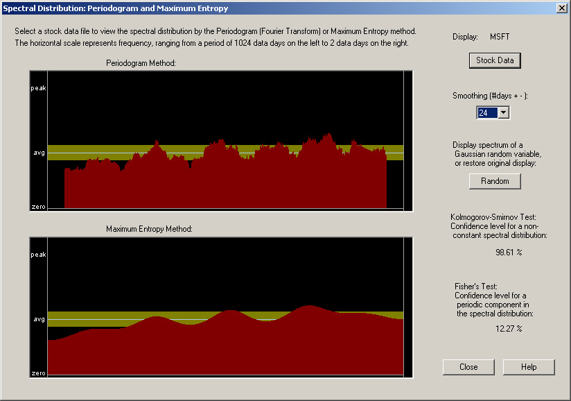
We see that this periodogram, when smoothed, bears some resemblance to the expected spectral density for the Fractional Difference filter with a negative fractional dimension. In particular, notice how it falls off at zero frequency, on the left-hand side. This is at variance with the expected behavior for a long-memory process with a positive fractional dimension, which should rise (in fact, go to infinity) at zero frequency. Notice also the fact that the Kolmogorov-Smirnov Test indicates a result that the confidence level for a non-random spectral distribution is 98.61%. This provides evidence that there may indeed actually be real correlation present, although there is also a 1.4% probability that this could just be due to random chance.
It appears that the excellent results obtained here from the Fractional Difference filter with a negative fractional dimension have nothing to do with fractal statistics per se, but are just due to the fact that this filter describes anti-persistence. (Persistence means that the spectrum rises at low frequencies and falls off at high frequencies. Anti-persistence means the spectrum is low at low frequencies and rises at high frequencies.) Any filter, such as the Linear Prediction filter, adapted to a spectral density which is low at low frequencies and rises for higher frequencies might do the job. In fact, the bottom pane of the above spectrum, labeled Maximum Entropy Method, is nothing other than the spectrum estimated from the filter coefficients of the Linear Prediction filter (see Numerical Recipes). So perhaps a kind of hybrid filter, combining a Linear Prediction filter in which the coefficients are smoothed (corresponding to the smoothed spectral density shown above) with the Fractional Difference filter, would be the optimum solution. In any event, the spectral density of each stock appears to be different, so the filter will have to be adapted to each stock, and will probably vary with time as well.
References
Peter J. Brockwell & Richard A. Davis, Time Series: Theory and Methods, 2nd ed., Springer-Verlag, New York (1991)
Edgar E. Peters, Chaos and Order in the Capital Markets, John Wiley & Sons, Inc., New York, NY (1991)
Edgar E. Peters, Fractal Market Analysis, John Wiley & Sons, Inc., New York, NY (1994)
William H. Press, Saul A. Teukolsky, William T. Vetterling, & Brian P. Flannery (NR), Numerical Recipes in C, The Art of Scientific Computing, 2nd ed., Cambridge University Press, Cambridge, UK (1992)
return to Demonstrations page